Building Neural Networks From Scratch

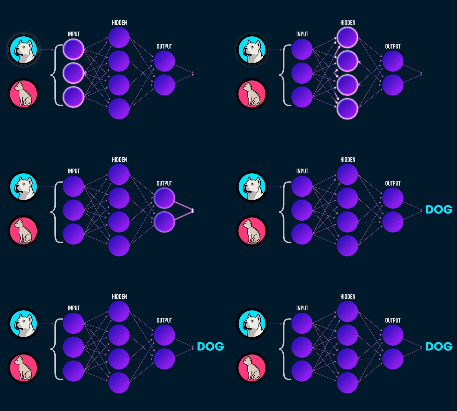
I’d been using TensorFlow for a while, but honestly had no clue what was actually happening behind all those convenient functions. So I decided to build a neural network using just NumPy to really understand the math. Shoutout to Michael Nielsen’s book and 3Blue1Brown’s videos for making the concepts click.

What We’re Building

A neural network is basically just layers of neurons doing matrix math with some nonlinear functions thrown in. Each neuron takes inputs, multiplies them by weights, adds a bias, and spits out a number:

$$z=\sum_{i=1}^{n}w_ix_i+b$$

Let’s build a simple three layer network to see how this works:

import numpy as np

class NeuralNetwork:
    """
    Neural network implementation using only NumPy.
    Supports arbitrary layer dimensions with sigmoid activation.
    
    Attributes:
        layer_dims: Dimensions of each network layer
        parameters: Network weights and biases
    """
    def __init__(self, layer_dims: list[int]) -> None:
        """
        Initialize network with specified layer dimensions
        
        Args:
            layer_dims: List of integers specifying nodes in each layer
        """
        self.layer_dims = layer_dims
        self.parameters = self._initialize_parameters()

Setting Up the Weights

Here’s something I learned the hard way: how you initialize your weights actually matters a lot. If they’re too big or too small, your network either explodes or barely learns anything. Xavier initialization helps keep things reasonable:

def _initialize_parameters(self) -> dict[str, np.ndarray]:
    """
    Initialize network parameters using Xavier initialization
    
    Returns:
        Dictionary containing weights (W) and biases (b) for each layer
    """
    parameters: dict[str, np.ndarray] = {}
    
    for l in range(1, len(self.layer_dims)):
        parameters[f"W{l}"] = np.random.randn(
            self.layer_dims[l], 
            self.layer_dims[l-1]
        ) * np.sqrt(1./self.layer_dims[l])
        parameters[f"b{l}"] = np.zeros((self.layer_dims[l], 1))
    
    return parameters

Forward Pass

This is where we actually run data through the network. We use the sigmoid function to squash outputs between 0 and 1:

$$\sigma\left(z\right)=\frac{1}{1+e^{-z}}$$

Here’s how that looks in code:

def forward_propagation(
    self, 
    X: np.ndarray
) -> tuple[np.ndarray, dict[str, np.ndarray]]:
    """
    Compute forward pass through the network
    
    Args:
        X: Input data of shape (input_size, m) where m is batch size
        
    Returns:
        Tuple containing:
            - Output activations
            - Cache of intermediate values for backpropagation
    """
    cache: dict[str, np.ndarray] = {}
    A = X
    
    for l in range(1, len(self.layer_dims)):
        Z = np.dot(self.parameters[f"W{l}"], A) + self.parameters[f"b{l}"]
        A = 1/(1 + np.exp(-Z))
        cache[f"A{l}"] = A
        cache[f"Z{l}"] = Z
    
    return A, cache

Measuring How Wrong We Are

For binary classification, we use binary cross entropy loss. It basically punishes confident wrong answers more than uncertain ones:

$$E = -\frac{1}{m}\sum_{i=1}^m\left[y_i\log(a_i) + (1-y_i)\log(1-a_i)\right]$$

The math looks scary, but the idea is simple: we want our loss to get smaller as our predictions get better.

Learning Through Mistakes

The network learns by figuring out how much each weight contributed to the error, then adjusting accordingly. This uses the chain rule from calculus:

$$\frac{\partial E}{\partial w_i} = \frac{\partial E}{\partial y} \cdot \frac{\partial y}{\partial z} \cdot \frac{\partial z}{\partial w_i}$$

Once we have these gradients, we update the weights:

$$w_i := w_i - \alpha \frac{\partial E}{\partial w_i}$$

Here’s the training loop:

def train(
    self, 
    X: np.ndarray, 
    Y: np.ndarray, 
    learning_rate: float = 0.1, 
    epochs: int = 1000
) -> list[float]:
    """
    Train the network using gradient descent
    
    Args:
        X: Training data of shape (input_size, m)
        Y: Target values of shape (output_size, m)
        learning_rate: Step size for gradient descent
        epochs: Number of training iterations
        
    Returns:
        List of training losses per epoch
    """
    losses: list[float] = []
    m = X.shape[1]
    
    for _ in range(epochs):
        A, cache = self.forward_propagation(X)
        loss = -1/m * np.sum(Y * np.log(A) + (1-Y) * np.log(1-A))
        losses.append(float(loss))
        
        self._backward_propagation(X, Y, cache, learning_rate)
    
    return losses

The Backpropagation Algorithm

This is where the real magic happens. We work backwards through the network, figuring out how much each parameter contributed to the final error. For the output layer, it’s straightforward:

$$\frac{\partial L}{\partial z^{[L]}} = A^{[L]} - Y$$

For hidden layers, we need to use the chain rule:

$$\frac{\partial L}{\partial z^{[l]}} = W^{[l+1]T} \frac{\partial L}{\partial z^{[l+1]}} \odot \sigma’(z^{[l]})$$

Here’s the implementation:

def _backward_propagation(
    self,
    X: np.ndarray,
    Y: np.ndarray,
    cache: dict[str, np.ndarray],
    learning_rate: float
) -> None:
    """
    Compute gradients and update network parameters
    
    Args:
        X: Input data of shape (input_size, m)
        Y: Target values of shape (output_size, m)
        cache: Dictionary containing intermediate values from forward pass
        learning_rate: Step size for gradient descent
    """
    m = X.shape[1]
    L = len(self.layer_dims) - 1
    
    dA = -(np.divide(Y, cache[f"A{L}"]) - 
           np.divide(1 - Y, 1 - cache[f"A{L}"]))
    
    for l in reversed(range(1, L + 1)):
        Z = cache[f"Z{l}"]
        A_prev = cache[f"A{l-1}"] if l > 1 else X
        
        dZ = dA * (cache[f"A{l}"] * (1 - cache[f"A{l}"]))
        
        dW = 1/m * np.dot(dZ, A_prev.T)
        db = 1/m * np.sum(dZ, axis=1, keepdims=True)
        
        self.parameters[f"W{l}"] -= learning_rate * dW
        self.parameters[f"b{l}"] -= learning_rate * db
        
        if l > 1:
            dA = np.dot(self.parameters[f"W{l}"].T, dZ)

The gradients for weights and biases work out to:

$$\frac{\partial L}{\partial W^{[l]}} = \frac{1}{m}\frac{\partial L}{\partial z^{[l]}}A^{[l-1]T}$$

$$\frac{\partial L}{\partial b^{[l]}} = \frac{1}{m}\sum_{i=1}^m \frac{\partial L}{\partial z_i^{[l]}}$$

Putting It All Together

A few things I learned while implementing this:

The gradient calculations work on entire batches at once, which makes everything much faster. We also save the intermediate values during the forward pass so we don’t have to recalculate them later. And here’s a nice trick: the derivative of sigmoid has a really clean form: $\sigma’(z) = \sigma(z)(1-\sigma(z))$.

That’s pretty much it. The network keeps doing forward passes to make predictions, then backward passes to learn from mistakes. Over time, it gets better at whatever task you’re training it on. Building this from scratch really helped me understand what all those TensorFlow functions are actually doing under the hood.